Loss of North American Freshwater Biodiversity

By Chris Schenker, SRC intern

Despite garnering less attention than their marine counterparts, freshwater species are diverse, important, and also under threat. Despite covering only 0.8% of the world’s surface and accounting for about 0.01% of the world’s water, freshwater contains at least 100,000 distinct species (Dudgeon et al. 2006). Comparisons to other environments are difficult because of the variation surrounding estimates of the total number of species on Earth. However, given freshwater’s disproportionately small share of total volume and surface area, it is beyond doubt to assert that its species density is staggeringly high. Although the interrelationships are not completely understood, freshwater biodiversity plays a crucial in ecosystem function as a whole. Despite the value that freshwater flora and fauna add from a scientific, commercial, aesthetic, cultural, and recreational perspective, the species extinction rate is far higher than that for their terrestrial counterparts (Dudgeon et al. 2006).

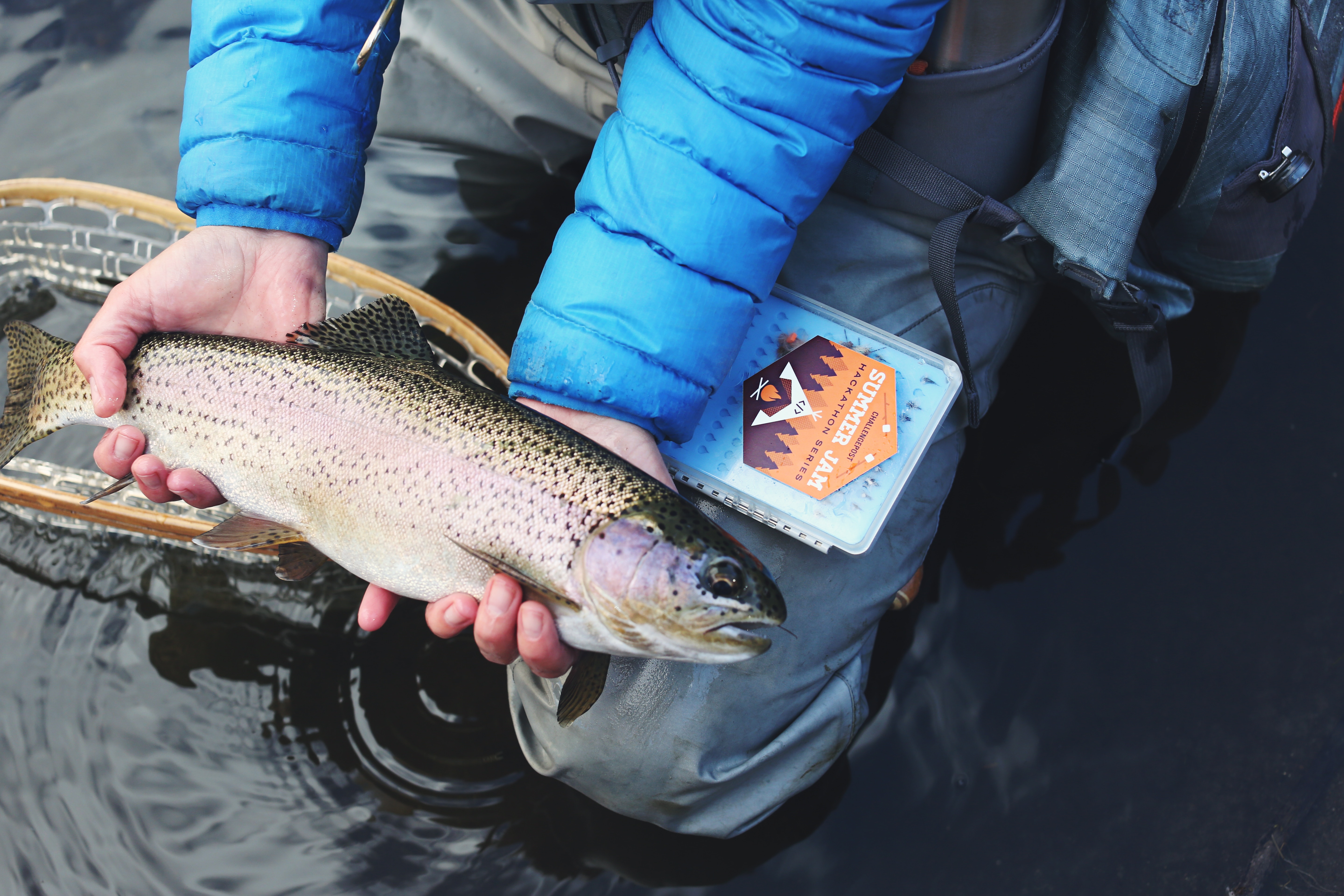
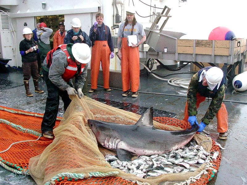
Figure 1: Freshwater fish are under threat worldwide, but the trend is especially pronounced in North America. (Unsplash.com)

This dynamic is especially clear in North America, where aquatic environments are well-studied. Although freshwater biodiversity is higher in the tropics, North America has the highest nontropical species diversity (Lundberg et al. 2000), totaling 1,213 as of 2010 and accounting for 8.9% of the world’s freshwater fish species (Nelson et al. 2004). There is a long history of species documentation in North America, with the first observed extinctions occurring in the early twentieth century. Since then, 39 species of North American freshwater fish have been declared extinct (IUCN 2011), yielding a continental extinction rate of 3.2% (Burkhead 2012). This is a higher total than is observed globally, but that is only because of North America’s longer history of continuous faunal study in comparison to the tropics. Regions with similar histories of scientific documentation display similar trends, with 3.4% of species considered extinct in Europe (Freyhof and Brooks 2011), and 3.2% of species considered extinct in the European basin (Smith KG and Darwall 2006).

The metric that really matters is the modern extinction rate in comparison to the background extinction rate. The background extinction rate, often abbreviated BER, is the taxonomic extinction rate over geologic timescales before the introduction of human pressures. Knowing both values allows scientists to calculate the ratio of modern extinction rate to background extinction rate (M:BER). There are difficulties in calculating both rates, so numbers should be interpreted with a grain of salt, but this ratio gives a rough estimate of how much faster extinction is occurring due to humanity’s global remodeling. The M:BER ratio for North American freshwater fishes has been calculated to be as high as 877 (Burkhead 2012), making it the highest number for any contemporary vertebrate group (Barnosky et al. 2011). Despite the large number of estimates and assumptions underlying this number, it highlights the severity of the problem species are facing. Fishes labeled as threatened, endangered, and declining will be subjected to the most intense pressure, especially those that are endemic and lie in the path of future human expansion.

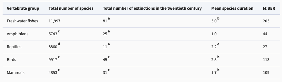
Figure 2: This table compares the modern extinction rates for world vertebrates to their estimated background extinction rates. (Burkhead 2012)

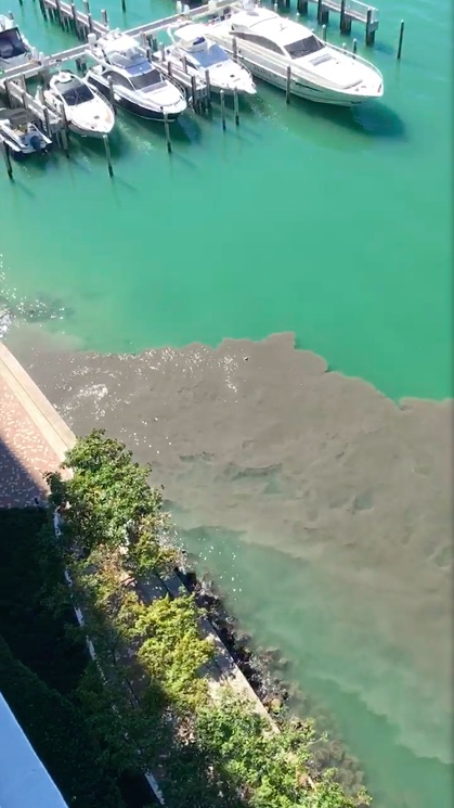
As imperiled as freshwater fishes are, they are only the beginning when it comes to declining freshwater flora and fauna. Many molluscs, such as snails and mussels, are going extinct at a rate that is an order of magnitude greater than that of freshwater fishes (Burkhead 2012). The main cause of this plight is human alteration of rivers and lakes, along with runoff, pollution, and the introduction of invasive species, such as zebra mussels (Cope et al. 2008). Mussels play an important role in their aquatic communities, such as providing habitat, filtering the water column, and depositing nutrients into the sediment. There is much scientific interest in what will happen to freshwater ecosystems as mussel species diversity and biomass declines.

The effect that mussels have on water filtration and waste recycling can vary widely based on the species, abundance, and environmental conditions present at the time. When water flow is low, such as in late summer, mussel communities can filter the entire volume. When water flow is high during times of melting and drainage, however, their effect is greatly reduced (Vaughn et al. 2004). Filtration performance is further affected by water temperature, with each species having its own optimal temperature. This means that in aquatic environments with multiple species of mussels, the ecosystem wide impacts of their filtration will vary widely based upon the relative dominance of each species, water flow, and temperature. Further complicating the equation is the fact that mussels also excrete ammonia, and their excretion rates can move in tandem with filtration rates, in the opposite direction, or not at all. It is all temperature dependent  (C.C. Vaughn 2010). The ammonia excreted by mussels plays an important role in lake and riverine ecosystems, boosting primary production and also benefiting consumers down the line (Spooner and Vaughn 2006). Even if excretion and filtration rates can be modeled for a set of known variables, it is important to remember that mussel communities can change in biomass and species dominance over time, and hydrological conditions are also dynamic.

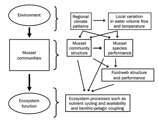
Figure 3: This conceptual model demonstrates the complicated interplay between mussel species density, community structure, and ecosystem processes. (C.C. Vaughn 2010)

This example serves an important point. Attempting to understand how an aquatic environment will respond to changes in species composition is difficult. With so much uncertainty about the effects of biodiversity loss in North American freshwater ecosystems, we as a society have no idea what we may be getting ourselves in for. It is therefore prudent to prioritize the conservation of at-risk populations so that we do not have to contend with the damage that their losses may entail.

Works Cited

Dudgeon, David & Arthington, Angela & Gessner, Mark & Kawabata, Zen-Ichiro & Knowler, D & Lévêque, Christian & J Naiman, Robert & Prieur-Richard, Anne-Hélène & Soto, D & Stiassny, Melanie & A Sullivan, Caroline. (2006). Freshwater Biodiversity: Importance, Threats, Status and Conservation Challenges. Biological reviews of the Cambridge Philosophical Society. 81. 163-82. 10.1017/S1464793105006950.

Lundberg JG Kottelat M Smith GR Stiassny MLJ Gill AC. 2000. So many fishes, so little time: An overview of recent ichthyological discovery in continental waters. Annals of the Missouri Botanical Garden  87: 26–62.

Nelson JS Crossman EJ Espinosa-Pérez H Findley LT Gilbert CR Lea RN Williams JD. 2004. Common and Scientific Names of Fishes from the United States, Canada, and Mexico, 6th ed.

American Fisheries Society. Special Publication no. 29.

[IUCN] International Union for Conservation of Nature. 2011. IUCN Red List of Threatened Species, version 2011.2. IUCN. (13 June 2012; www.iucnredlist.org)

Freyhof J Brooks E. 2011. European Red List of Freshwater Fishes. Publications Office of the European Union.

Smith KG Darwall WRT eds. 2006. The Status and Distribution of Freshwater Fish Endemic to the Mediterranean Basin. International Union for the Conservation of Nature. (14 June 2012; http://data.iucn.org/dbtw-wpd/html/Red-medfish/cover.html)

Noel M. Burkhead, Extinction Rates in North American Freshwater Fishes, 1900–2010, BioScience, Volume 62, Issue 9, September 2012, Pages 798–808, https://doi.org/10.1525/bio.2012.62.9.5

Barnosky AD et al. .2011. Has the Earth’s sixth mass extinction already arrived? Nature 471: 51–57.

Cope WG et al.  2008. Differential exposure, duration, and sensitivity of unionoidean bivalve life stages to environmental contaminants. Journal of the North American Benthological Society 27: 451–462.

C.C. Vaughn. Biodiversity losses and ecosystem function in freshwaters: emerging conclusions and research directions. Bioscience, 60 (2010), pp. 25-35, 10.1525/bio.2010.60.1.7

Vaughn CC Gido KB Spooner DE. 2004. Ecosystem processes performed by unionid mussels in stream mesocosms: Species roles and effects of abundance. Hydrobiologia 527: 35–47.

Vaughn CC Spooner DE. 2006. Unionid mussels influence macroinvertebrate assemblage structure in streams. Journal of the North American Benthological Society  25: 691–70

Permeable Pavement Systems as a Mitigation Strategy to Combat Stormwater Outfall and Sea Level Rise

By Casey Dresbach, SRC intern

The EPA defines stormwater runoff as that which is generated from rain events that flow over land or impervious surfaces, such as paved streets, parking lots, and building rooftops, and does not soak into the ground (EPA, 2018). This accumulation of water ultimately ends up in coastal waters, but upon its journey it picks up a plethora of pollutants ranging from trash, chemicals, fecal matter, and sediment. These substances picked up by the runoff are compromising the health and water quality of these waters. A large portion of the global warming heat is accumulating in oceans worldwide. As a result, sea levels are rising through thermal expansion of water in the oceans and melting of ice sheets and glaciers on land.

Between 1998 and 2006 alone, tidal gauges showed sea levels in South Florida followed average global rate (0.04 to 0.20 inches per year) – but in 2006, local rates suddenly underwent a rapid acceleration, averaging about 0.20 inches to a half inch each year (Staletovich, 2016). Over the last decade, flood management has become increasingly important to several coastal states at risk such as Florida, Louisiana, New York, and California with each region varying in susceptibility to sea level rise. Flood management is commonly issued by drainage systems such as complex pipe networking. However, these projects are extremely costly and only seem to be dealing with the issue on a short-term basis. These stormwater controls are known as best management practices (BMPs) intended to filter out pollutants. Miami Beach has already undergone a major BMP using “gray stormwater infrastructure,” that is their $500 million drainage and water treatment system, one of which resides in a highly populated area (Harris, 2018). This coastal area, also known as Sunset Harbor Village, is home to local businesses, restaurants, bars, and boutique fitness enterprises. Yet, the effectiveness is not justifying the efforts taken to mitigate the impacts of sea level rise and urban development. The pump fails to filter out many of these pollutants pervading the streets and they ultimately end up into the coastal waters of Biscayne Bay (Figure 1).

Figure 1. Dirty Water Pumped Into Biscayne Bay (Caption: Dirty water pumped into Biscayne Bay in Miami Beach, FL. Snapshot from video taken by Miami Beach citizen.  (Lipscomb, 2019))

Benjamin O. Brattebo and Derek B. Booth conducted a study to examine the long-term stormwater quantity and quality performance of permeable pavement systems. Permeable pavement is made up of a matrix of concrete blocks or plastic structure with holes filled with sand, gravel or soil (Brattebo & Booth, 2003). The filling absorbs the outfall that might otherwise percolate into alternative places, most notably are coastal environments. The voids allow stormwater to seep through the pavement and into the soil. Asphalt pavement, an impervious system, was compared to four permeable pavements created in a monitored and controlled parking lot in Renton, Washington. Employees of King County Public Works facility utilize the parking facility during the workweek, Monday through Friday. Plastic Grasspave, plastic Gravelpace, concrete Turfstone, and concrete UNI Eco-stone were the permeable systems used. The first two plastic grids differed in their fill. The first was filled with sand and planted with grass and the second was filled with gravel only. Similarly, the first concrete was filled with soil and planted with grass while the latter was filled with gravel. Each permeable pavement had two parking stalls paired into one instrument station (Brattebo & Booth, 2003), which made up 8 stalls. The ninth stall was the asphalt-paved control. See Figure 2. During 15-minute rainfall events, runoff rates were cataloged. Water was collected and sampled in both the impermeable and permeable systems. Surface durability, infiltration capacity, and water-quality performance were assessed. Results showed that overall samples from permeable systems contained overwhelmingly lower levels of copper and zinc, and none had traces of diesel fuel or lead. Researchers indicated that while their findings support long-term success for infiltration via permeable systems, the success might not be universal in places with extremely arid or colder snow induced climates.

Figure 2. Plan View of 9 Parking Stalls JPEG aligned center. (Caption: 8 impermeable systems installed in parking lot alongside 1 control, the permeable asphalt concrete system. (Brattebo & Booth, 2003))

More research needs to be done in order to combat the challenges that arise with stormwater runoff and urban redevelopment continues on an upward trend. Long-term solutions and studies are crucial but as are short-term. A perfect balance of the two will help mitigate the detrimental impacts of pollutants trickling into larger water bodies that are utilized by the overall marine ecosystem, humans and coastal fauna included.

Works Cited

Brattebo, B. O., & Booth, D. B. (2003). Long-term stormwater quantity and quality performance of permeable pavement systems. Water Research , 37 (18), 4369-4376.

EPA. (2018, September 14). NPDES Stormwater Program. Retrieved from EPA: https://www.epa.gov/npdes/npdes-stormwater-program

Harris, A. (2018, April 18). Miami Beach’s future is ‘uncertain,’ experts say, but sea rise pumps are a good start. (Miami Herald) Retrieved March 20, 2019, from Miami Herald: Miami Beach’s future is ‘uncertain,’ experts say, but sea rise pumps are a good start: http://www.miamiherald.com/news/local/community/miami-dade/miami-beach/article209328849.html#storylink=cpy

Lipscomb, J. (2019). Videos Show Dirty Stormwater Pumped Into Biscayne Bay and Swallowed by Manatee. (M. N. Times, Producer) Retrieved from Miami New Times: https://www.miaminewtimes.com/news/videos-show-dirty-stormwater-pumped-into-biscayne-bay-and-swallowed-by-manatee-11068892

Staletovich, J. (2016, April 7). Miami Beach flooding spiked over last decade, UM study finds. (Miami Herald) Retrieved April 30, 2018, from Miami Herald: http://www.miamiherald.com/news/local/environment/article70145652.html

A microscopic organism with a macroscopic impact: How climate change is affecting harmful algal blooms and what this means for future generations

By Carolyn Hamman, SRC intern

Phytoplankton are photosynthetic microorganisms that exist in both marine and freshwater environments. There are several different types of phytoplankton each with their own unique preferred environmental parameters and strategies for growth. For example, some phytoplankton (called coccolithophores) use calcium to create protective plates they use as a defense mechanism (Beaufort et al. 2011). Phytoplankton are a vital component in aquatic ecosystems as they are responsible for the majority of primary productivity that occurs. In fact, phytoplankton have been considered a driver in climate as 30% of anthropogenic carbon emissions have been absorbed by the ocean and over 90% of the heat increase the Earth has seen the ocean has taken up (Hallegraeff 2010). While phytoplankton plays a vital role in many processes in the ocean, there are also occurrences of harmful algal blooms (HABs). HABs are phenomena that have been a natural process throughout history (Hallegraeff 2010). These blooms can be harmful for two reasons. Certain species of phytoplankton can produce different types of neurotoxins that have been known to cause different problems such as respiratory issues (such as with the Florida Red Tides) or gastrointestinal and neurological illnesses. HABs don’t have to necessarily produce toxins to be considered harmful. The dense covering that algal blooms can cause blocks UV light from reaching certain depths of the ocean. The high amount of phytoplankton will cause a depletion in nutrients that can disrupt other ecosystems who rely on the nutrients as well. Once the phytoplankton finally use up the nutrients, they die in massive amounts that deplete the oxygen in the water and causes massive anoxia (Hallegraeff 2010).

Climate refers to the large-scale changes that occur in the atmosphere, hydrosphere, and cryosphere (Hallegraeff 2010). There are natural fluctuations in the climate that have caused periods of warming or cooling. However, since around the Industrial Revolution, the CO2 levels have increased from 280 to >380 ppm, and there have been temperature increases in the past 40 years that are at a rate far faster than ever seen before (Hallegraeff 2010). Phytoplankton have short generation times and longevity, which means they can respond quickly to climate change. This is true for HABs as well. Though phytoplankton species can evolve and change, the changing environmental parameters will favor species with certain parameters. As climate continues to change, it is imperative to understand how HAB will respond. The issue is that there are numerous amounts of factors that all play a role in determining which species of algae bloom (Zingone & Enevoldsen 2000). These stressors caused by climate change can include increased temperature, enhanced surface stratification, alteration of ocean currents, intensification or weakening of nutrient upwelling, stimulation of photosynthesis by elevated CO2, reduced calcification from ocean acidification, and changes in land runoff and micronutrients (Hallegraeff 2010). Each of these parameters can be analyzed to determine how HAB will respond to climate change. In the past 30 years, there has been an increase in frequency and intensity of HAB as well as how widespread they are (Hallegraeff 2010).

As greenhouse gas concentrations have increased there has been an increase in surface temperature, lower pH, and changes in vertical mixing, upwelling, precipitation, and evaporation patterns (Moore et. al. 2008). As current strength and number of blooms have increased, the range of HAB has expanded (Hallegraeff 2010). Areas that had previously not seen HAB have noticed a significant increase in the past decade. HAB rely on temperature to bloom, and with an increase in overall temperature blooms have started to occur earlier than what has previously been observed (Hallegraeff 2010). Phytoplankton living in shallower areas will also be more effected by temperature than phytoplankton in open oceans (Hallegraeff 2010). This means that HAB closer to the shore will undergo larger changes than the populations in the open ocean. With increased greenhouse gases comes increase in sea-level, wind, and mixed-layer depth, which has an impact on the number of upwelling and downwelling events and thus concentrations of macronutrients (Hallegraeff 2010). The change in wind will also influence transport of nutrients by air (known as aeolian transport). The net result is a decrease in mixing depth at higher latitudes, which results in higher phytoplankton biomass (Hallegraeff 2010). A noticeable change in precipitation is occurring due to climate change as well, where there are now periods of concentrated rainfall followed by long dry spells. This change is causing certain dinoflagellates (a type of phytoplankton) to bloom in higher concentrations than previously seen before (Hallegraeff 2010).

A schematic showing how climate warming affects mixing in low and high latitudes. The differences in mixing results in differences in HAB (Hallegraeff 2010)

The environmental changes caused from climate change has caused HAB patterns not previously seen before. Going in to the future, the species-specific responses to these parameters can be used to better predict where HAB will occur and the concentration they could occur at. The potential issue with such predictions is that it is exceedingly difficult to be able to predict how several environmental parameters working together will cause phytoplankton to respond. It is recommended that there be a more improved global ocean observation system that can monitor all of these parameters simultaneously (Hallegraeff 2010). As previously mentioned, there could be increased adverse effects on human health due to increased HAB, but very little has been done to study how humans respond to different phytoplankton toxins (Moore et. al. 2008). More research is needed to evaluate associations between human health and HAB to better respond when harmful algal bloom occurrence continues to increase in to the future.

A graph showing the relationship between the number of algal blooms and human population over time. Populations and boom frequency have both increased over time (Zingone & Enevoldsen 2000)

Works cited

Beaufort, L., Probert, I., De Garidel-Thoron, T., Bendif, E. M., Ruiz-Pino, D., Metzl, N., … & Rost, B. (2011). Sensitivity of coccolithophores to carbonate chemistry and ocean acidification. Nature476(7358), 80.

Hallegraeff, G. M. (2010). Ocean Climate Change, Phytoplankton Community Responses, And Harmful Algal Blooms: A Formidable Predictive Challenge. Journal of Phycology, 46(2), 220-235. doi:10.1111/j.1529-8817.2010.00815.x

Moore, S. K., Trainer, V. L., Mantua, N. J., Parker, M. S., Laws, E. A., Backer, L. C., & Fleming, L. E. (2008). Impacts of climate variability and future climate change on harmful algal blooms and human health. Environmental Health, 7(S4), 1-12. doi:10.1186/1476-069x-7-s2-s4

Zingone, A., & Enevoldsen, H. O. (2000). The diversity of harmful algal blooms: A challenge for science and management. Ocean & Coastal Management, 43(8-9), 725-748. doi:10.1016/s0964-5691(00)00056-9

A Summary of Acoustic Tagging and Juvenile Salmon Acoustic Telemetry System Program in the Northwestern United States

By Brenna Bales, SRC intern

Before the existence of satellite and acoustic tracking technologies, the most we knew about a certain marine species’ range was from either visual observations or catch data. By developing these systems and scientists cooperating globally by sharing their data, we have learned that some “tropical” species like tiger sharks are not tropical at all but can in fact go as far north as Maine or Canada and out thousands of miles into the mid-Atlantic on a single migration from Florida (sharktagging.com). In 1999, an estimated 11,800 electronic tags (both satellite and acoustic) were placed on marine mammals, fish, invertebrates, reptiles, and birds around the world (Stone et al, 1999). There is a major difference between these two technologies, however. While satellite tags will track an animal wherever it goes as long as it can communicate with a satellite (meaning the tag must hit the surface to be detected), acoustic tags (Image 1) must be within range to an underwater hydrophone for the signal to be detected. This enables acoustically tagged animals to be tracked on a much finer scale without the need for the animal to come to the surface.

Image 1: Differently sized acoustic tags that would be used internally to monitor movements of animals.

A research organization may set up a hydrophone array over a certain area to pinpoint their tagged animals’ locations; however, this array may also detect other animals that have been acoustically tagged by different research organizations. This can be helpful to everyone, as only one hydrophone is needed to track all kinds of animals and their tags, such as sawfish, sharks, and marine mammals; however, private interests may hinder this (Grotheus 2009). Lastly, acoustic tagging has benefits in that it can be used to track multiple individuals within a population in one location versus a small number of animals tracked over different time scales and locations (Huepel et al, 2006).

In 2001, the U.S. Army Corps of Engineers Portland District decided that they wanted to track juvenile salmon in the Columbia river basin through their migration to the Pacific Ocean. There were several goals to the JSATS (Juvenile Salmon Acoustic Telemetry System) project, including 1) assessment of survival and habitat use of juvenile salmonids migrating through the estuarine environment 2) estimation of route-specific dam passage survival of juvenile salmonids 3) determination of fish survival and migration behavior, and 4) to determine effects of water temperature stratification and dissolved gas (https://waterpower.pnnl.gov/jsats/). By 2008, 4,140 JSATS  and 48,433 passive integrated transponder (PIT)- tagged yearling Chinook salmon (Oncorhynchus tshawytscha) had been tagged (McMichael et al, 2010). The dams are shown in Image 2 along with the route that the salmon migrated towards the Pacific Ocean.

Image 2: Study area used in JSATS in the Snake and Columbia river basins in 2008. Red circles demarcate the hydrophone array locations and the star marks the release location of the tagged yearling Chinook salmon.

The researchers on the project concluded that the JSATS tags gave more survival location data with higher precision than the PIT tags (McMichael et al, 2010). The JSATS tags also transmitted every 5 seconds, which is optimal for the current study in tracking such small-scale movements around the local dams. All components of the system were non-proprietary, unlike many other arrays currently established. A major outcome from this was the competitive nature in which the U.S. Army Corps of Engineers bid for reductions in sizing and pricing for these tags, leading to many advances in the technology. The study is on-going, and research is being conducted on the biological effects of tagging and how the environment is affecting the receivers and their detection capability. This telemetry system has been designed extremely efficiently and should be used as a model for other up and coming acoustic tagging endeavors.

Literature Cited

Grothues, T.M., 2009. A review of acoustic telemetry technology and a perspective on its diversification relative to coastal tracking arrays. In Tagging and tracking of marine animals with electronic devices (pp. 77-90). Springer, Dordrecht.

Heupel, M.R., Semmens, J.M. and Hobday, A.J., 2006. Automated acoustic tracking of aquatic animals: scales, design and deployment of listening station arrays. Marine and Freshwater Research, 57(1), pp.1-13.

McMichael, G.A., Eppard, M.B., Carlson, T.J., Carter, J.A., Ebberts, B.D., Brown, R.S., Weiland, M., Ploskey, G.R., Harnish, R.A. and Deng, Z.D., 2010. The juvenile salmon acoustic telemetry system: a new tool. Fisheries, 35(1), pp.9-22.

Stone, G., Schubel, J. and Tausig, H., 1999. Electronic marine animal tagging: New frontier in ocean science. OCEANOGRAPHY-WASHINGTON DC-OCEANOGRAPHY SOCIETY-, 12, pp.24-27.

Image 1 source: https://commons.wikimedia.org/wiki/File:Example_of_Acoustic_Telemetry_Tags_for_Fisheries_Research.jpg

Image 2: McMichael, G.A., Eppard, M.B., Carlson, T.J., Carter, J.A., Ebberts, B.D., Brown, R.S., Weiland, M., Ploskey, G.R., Harnish, R.A. and Deng, Z.D., 2010. The juvenile salmon acoustic telemetry system: a new tool. Fisheries, 35(1), pp.9-22.

Migration Dynamic of Juvenile Southern Bluefin Tuna

By: Julia Saltzman, SRC Intern

Large-scale migrations are crucial to many different marine species. In southern bluefin tuna, this life history trait is critical for sustaining their valuable fisheries, and as such there are many scientific research programs designed to monitor the management of the species. Telemetry technology (remote tracking of spatial locations and movements) has made cycles more generally observable, however quantifying variability and plasticity of migration schedules still remains a challenge. In this study from Patterson et al. (2018), movements from 110 individual juvenile southern bluefin tuna were estimated from the period of 1998-2011. The authors found that individuals demonstrated considerable variability in migratory patterns between the years. Patterns observed that juvenile southern bluefin tuna progressively spent less time in shelf waters, and the moved east, rather than west into the Tasman Sea for a higher period then heading west into the India Ocean. In addition, it was found that the further southern bluefin tuna move from the Great Australian Bight (GAB), the more time they spend migrating. This study also determined three areas associated with the residency of juvenile southern bluefin tuna. These areas of residence were far different from the known areas of residence in the past. The productivity in these residency regions displayed a seasonal cycle.

This study asserted that much like other large marine animals who use temperate latitudes, juvenile southern bluefin tuna also undertake long distance and large-scale migrations. In addition, while fish were observed to migrate to key areas, their patterns, especially in the winter months, varied both on an individual and yearly basis. Researchers suggested that for fast growing, immature, large, predators, such as those studied here their migration may be related to environmentally availability, rather than cues which are fixed such as day length. Other environmental factors also impact the migrations; for example, because the fish is a visual predator, they prefer to hunt in clear waters away from areas of high turbidity and high primary productivity. In addition, it is likely that seasonal populations of small pelagic fish in the GAB coincide with the migration of the southern bluefin tuna.

Through the use of tag deployment and geolocation of juvenile southern bluefin tuna, and Hidden Markov Models to estimate when individuals were migrating, important insights were obtained on the individuals within the same period and within individuals across multiple years. The complexity of migration routes appears to be related to sea surface temperature, productivity, and the physiology of the individual southern bluefin tuna. This report provides scientists and fisheries managers with the information to effectively manage southern bluefin tuna. This species, which has faced massive declines in the past due to poor management strategies, is now much better managed due to an understanding of their varying migratory patterns, especially those of juveniles.

Work Cited:

Patterson, T. A., Eveson, J. P., Hartog, J. R., Evans, K., Cooper, S., Lansdell, M., … & Davies, C. R. (2018). Migration dynamics of juvenile southern bluefin tuna. Scientific reports8(1), 14553.

Climate Change Induced Trophic Amplification Declines Planktonic Biomass

By: Delaney Reynolds, SRC Intern

Figure 1: A collage of different planktonic organisms (Source: http://planktonchronicles.org/en/episode/plankton/)

Plankton, including phytoplankton and zooplankton, make up 99% of all marine life and form the base of the food web. Phytoplankton undergo photosynthesis, much like plants do, and thus their growth and population size are dependent on availability of nutrients and levels of light. Zooplankton feed upon phytoplankton and thus their population size is partly dependent on phytoplankton populations.

The effects of anthropogenic climate change on phytoplankton and zooplankton populations is widely unknown, but scientists are taking steps to determine what those effects may be.

In a study by the Dynamic Meteorology Laboratory in France, Dr. Lester Kwiatowski took a look at how the trophic amplification of plankton biomass changes based on different models of future climate change, as well as how an amplification of this response may trickle through the food web.

Two different modeling techniques were used in this study: the Coupled Model Intercomparison Project Phase 5 (CMIP5) Earth System Models and the Pelagic Interactions Scheme for Carbon and Ecosystem Studies Quota (PISCES-QUOTA) model. The CMIP5 models modeled the trophic interactions between zooplankton and phytoplankton biomass under twenty-first century climate change projections. The PISCES-QUOTA model was used to explore what the mechanisms controlling zooplankton and phytoplankton trophic interactions might be under different climatic conditions.

Figure 2: This figure displays the projected percentage of plankton biomass anomaly by year from 1850 to 2100, as well as according to latitude. All three populations of plankton (phytoplankton, microzooplankton, and mesozooplankton) decrease in biomass; however, it can be concluded that the zooplankton will be much more negatively affected than the phytoplankton. It can also be deduced that in the lower latitudes, where it is warmer, zooplankton will also be more negatively affected than phytoplankton (Lester et al. 2018).

Kwiatowski found that both models projected a decline in both in zooplankton biomass and phytoplankton biomass as a result of climate change, with a moderately larger decrease in zooplankton biomass than phytoplankton biomass. According to the CMIP5 models, phytoplankton biomass is expected to decline by 6.1 ± 2.5% and zooplankton biomass is expected to decline by 13.6 ± 3.0%. The PISCES-QUOTA model split up zooplankton into two groups: microzooplankton and mesozooplankton. This model found that phytoplankton biomass is expected to decline by 8.5%, microzooplankton biomass by 15.4%, and mesozooplankton biomass by 20.6%. Here again, a slightly greater decrease in zooplankton biomass can be found than phytoplankton biomass. The PISCES-QUOTA model also determined that the driving factor affecting the biomass levels was primarily the fact that “primary production decreases in equatorial and subtropical biomes due to stratification-driven reductions in nutrient availability” (Kwiatowski et al., 2018).

Looking at comparisons between carbon, nitrogen, and phosphorous stoichiometry, the discrepancy between phytoplankton and zooplankton can be explained. As a result of climate change, the PISCES-QUOTA model also predicted a decrease in the phytoplankton nitrogen content by 1.1% and phosphorous content by 6.4%, just in the twenty-first century. As zooplankton consume phytoplankton, this decrease of nitrogen and phosphorous in phytoplankton will ultimately lead to a decline in the growth efficiency of zooplankton and a decrease in the overall zooplankton population.

Phytoplankton and zooplankton comprise of the base of the marine food web and also produce about 50% of the earth’s oxygen. Without them, many larger organisms would be heavily impacted. Studies just like this one can help us better understand the future that our delicate food web may face under the threats of climate change and give us insight into how we might be able to combat the probable effects.

Works Cited

Kwiatkowski, L., Aumont, O., & Bopp, L. (2019). Consistent trophic amplification of marine biomass declines under climate change. Global change biology25(1), 218-229.

The Utility of Combining Stable Isotope and Hormone Analyses for Marine Megafauna Research

By: Olivia Wigon, SRC Intern

Marine megafauna face many threats such as ship strikes, climate change, ocean noise and habitat destruction, which have caused many populations to decline. Typically, conservation takes a reactive approach instead of a proactive one which makes it hard to maintain healthy populations of marine megafauna. Alyson H. Fleming and her team are working with stable isotope and hormone analysis to understand in a more in-depth way how megafauna, specifically cetaceans, pinnipeds and sea turtles, are responding to their ever-changing environments (Fleming et al. 2018). The team is looking at physiological biomarkers that can help explain an animal’s movements, nutrition, stress, health and reproductive information. This data can give scientists and conservationist enough time to react proactively to the issues marine megafauna are facing. For example, looking at the ratios of stable carbon and nitrogen in bulk tissues Fleming and her team can determine not only the animal’s habitat but also its trophic level. This is made possible because the carbon and nitrogen isotopes found in bulk tissue indicate the biogeochemistry in the base of the food web. In addition to looking at stable isotopes the team looked at hormone levels. Hormones connected to reproduction can reveal an animal’s maturity, sex, whether or not the animal is pregnant, birth rates, sex ratios and more. Along with reproductive hormones there are stress hormones which can show predator exposure and areas of nutritional deficits. There are also thyroid hormones that will show an animal’s nutritive levels.

Some of the challenges with this research is that different tissues and different isotopes have different half-lives. The half-life rate varies based on the rates of protein metabolism. It is important to note that a tissue type can have different half-life rates based on the species and individual. Hormone analysis on the other hand is typically similar across vertebrate species however, the physiological roles of each hormone can have a different role in each species. Despite these challenges this is a growing and developing field of study. Integrating the results of stable isotope analysis with hormone analysis can answer many questions among many biological levels. When trying to solve a conservation issue it is best to have several lines of evidence which this process creates. Since this is a new and emerging field, there is still work to be done in regards to establishing methodology.

Work Cited:

Fleming, A. H., Kellar, N. M., Allen, C. D., & Kurle, C. M. (2018). The Utility of Combining Stable Isotope and Hormone Analyses for Marine Megafauna Research. Frontiers in Marine Science, 5, 1-15.


“Boo! Did we scare you?”: behavioral responses of reef-associated fish, prawn gobies (Amblyeleotris steinitzi and Amblyeleotris sungami) to anthropogenic diver disturbance 

By: Allison Banas, SRC Intern

There are many factors that can affect the health of coral reef communities, SCUBA diving being one of them. Studies have shown that divers’ activities can have significant detrimental effects on the ecosystem, and this paper from Valerio et al. (2018) looks at the effect divers can have on the behavior of two species of gobies.

The paper’s hypothesis is that divers in heavily dived areas have a habituating influence, along with causing a decreased latency period and a lower flight initiation distance (FID) on the gobies. This study took place at five sites along the Israeli coast of the Gulf of Eilat/Aqaba with differing levels of disturbance (Figure 1) Divers floated at least 3 m above the goby, and photographed the fish with a chosen scale object, and those gobies being disturbed were disturbed with a small weight attached to a nylon string wrapped around a pencil and lowered to land on the substrate approximately 15 cm in front of the goby. A timer was used to measure the latency period (time from disappearance to first reappearance), as soon as the goby retreated into its burrow. A seven-minute maximum time was pre-set.

Gobies in areas of high diver disturbance were found to no longer react to disturbances by having shorter latency periods, as well as shorter FID when compared to gobies at un-dived sites. Anthropogenic disturbance therefore is potentially leading to habituation of the gobies. The two different species of gobies were found to also have an effect on the data collecting, with A. sungami members having a significantly longer latency period than A. steinitzi, but this difference was found to be not significant. External factors including body size, circadian rhythm, depth and diving season were analyzed for significance, but none were found to have an effect on the latency periods.

This study opens the door for other studies to look at the potential effect of diver disturbance on the predation of gobies, since the gobies are spending less time in their burrows after a disturbance and have a shorter FID. If the same level of diver disturbance continues without rapidly habituating, the gobies could potentially spend a larger proportion of daylight hours in their burrows. Various statistical tests were completed in order to calculate potential diver effect, correlation between variables, average latency periods, and FID distances. In conclusion, diver disturbance has an effect on the behavior of gobies, and therefore the gobies have adapted their behavior.

Figure 1: A map showing the study sites along the coast of Eilat, Israel in the Gulf of Aqaba. (filled circle) Heavily dived (HD) and regularly dived (D); (light grey triangle) undived (UD); and relatively undived (RUD); and (light grey square) naturally disturbed (ND) [Dr. Gil Koplovitz]

Figure 2: Proportion of gobies that emerged over the 7-min time limit at each of the five sites. (Valerio et al. 2018)

Works cited

Valerio, M., Mann, O., & Shashar, N. (2019). “Boo! Did we scare you?”: behavioral responses of reef-associated fish, prawn gobies (Amblyeleotris steinitzi and Amblyeleotris sungami) to anthropogenic diver disturbance. Marine Biology166(1), 1.


Investigating the vulnerability of European Seafood Production to Climate Warming

By: Gaitlyn Malone, SRC Intern

As the world’s climate continues to change, economic, social, and environmental changes will undoubtedly occur along with it. One sector that is expected to be economically affected by climate warming is seafood production (Breitburg et al., 2018). Seafood production, which includes both farmed and captured fish, shellfish, and seaweed in marine and freshwater, will experience changes since the warming of an environment has the ability to change both a species’ distribution and life history characteristics (Pecl et al., 2017; Cochrane et al., 2009). Therefore, it is crucial to work towards being able to predict and understand the extent of these changes in order to prepare for the future.

A recent study (Blanchet et al., 2019) examined the effects of climate change on seafood production within each European country in order to identify potential challenges and opportunities within the sectors of marine fisheries, marine aquaculture, and freshwater production. To do so, the researchers combined information on the target species’ temperature preferences, life history characteristics, and production volume to determine their biological sensitivity (BS) and the maximum temperature (Tmax) that they were experiencing. They then determined the adaptive ability of seafood production in each country or sector by determining the number of species that the country/sector exploits and those species’ temperature ranges. A country or sector that exploits a higher number of species will be more likely to adapt in response to climate change. A species with a wide temperature range would also potentially be more adaptable since they are able to withstand a variety of temperatures.

Figure 1: Biological sensitivity index versus the temperature range of each species within the sectors of a) marine fisheries, b) marine aquaculture, and c) freshwater production. The size of the bubbles relates to the total volume produced for each particular species in that sector (Blanchet et al., 2019).

Figure 2: Ranking of each European country’s vulnerability to warming based on their weighted temperature sensitivity and weighted biological sensitivity for each of the three production sectors. The size of the bubbles represents the relative contribution of each country to the total European production volume within that sector (Blanchet et al., 2019).

Overall, seafood production was found to generally be more vulnerable within the marine fisheries and aquaculture sectors. The freshwater sector varied greatly based on country. Within the marine sector, northern countries tended to be more sensitive to warming than southern countries since seafood production in these areas are more dependent on cold-water species with a high BS. Southern countries tended to rely on warmer water species that had a lower BS. The main challenge facing these marine fisheries is due to changes in species distribution. In response to warming, there has been a northward expansion of the range of several species, which in some cases has included a contraction of their southern range. This change in distribution has the ability to affect local fisheries and management, who in southern areas may lose access to their resources, while northern areas may benefit. Aquaculture taking place in temperate zones was also predicted to be at risk from warming conditions, since increasing temperatures have the ability to reduce oxygen levels in the water and increase the metabolic costs for organisms. Disease is also likely to increase in these systems since pathogens may spread more readily. The low amount of species diversity in aquaculture also makes it particularly susceptible to rising temperatures.

Under warming conditions is not impossible to continue producing sustainable seafood, however efforts must be made to adapt to climate change. Therefore, the authors suggest that there must be communication between stakeholders, diversification of exploited species, and transnational cooperation in order to meet these goals.

Work Cited

Blanchet, M.-A., Primicerio, R., Smalas, A., Arias-Hansen, J., Aschan, M. 2019. How vulnerable is the European seafood production to climate warming?. Fisheries Research 209, 251-258.

Breitburg, D., Levin, L.A., Oschlies, A., Gr.goire, M., Chavez, F.P., Conley, D.J., Gar.on, V., et al., 2018. Declining oxygen in the Global Ocean and coastal waters. Science 359 (6371).

Cochrane, K., Young, D.C., Soto, D., Bahri, T., 2009. Climate change implications for fisheries and aquaculture: overview of current scientific knowledge. FAO Fisheries and Aquaculture Technical Paper 530, 212.

 Pecl, G.T., Ara.jo, M.B., Bell, J.D., Blanchard, J., Bonebrake, T.C., Chen, I.-C., Clark, T.D., et al., 2017. Biodiversity redistribution under climate change: impacts on ecosystems and human well-being. Science 355.


Effectiveness of MPA’s

By: Peter Aronson, SRC Intern

One might think that setting aside marine protected areas (MPA’s) – areas of the ocean where human activity is more heavily restricted – would reduce fishing pressure and overexploitation of marine species. However, that is not always the case. A group of researchers sought to determine if MPA’s experience intense human pressure, and if that pressure was undermining the goal of conserving biodiversity. They focused on European waters, where a substantial amount of industrial fishing occurs (Kroodsma et al., 2018), and an ample network of MPA’s covers about 29% of the sea (European Union, 2016).

Trawling is the most common method of industrial fishing in Europe (Kroodsma et al., 2018). It often has high bycatch rates and is a threat to many endangered species, including many elasmobranchs, as well as entire seafloor habitats. Researchers used satellite data to track fishing vessels and quantify commercial trawling effort. All 727 MPA’s in the study were considered 100% marine, designated prior to 2017, and listed on the World Database on Protected Areas.

Figure 1. Miramare Marine Reserve, Italy. (Sebastian Lake, September 29, 2015. Wiki Commons)

In 2017, combined trawling effort exceeded 1 million hours with over 225,000 occurring inside MPA’s. Trawling intensity, measured in hours per square kilometer, was 38% greater inside MPA’s compared to unprotected areas, and 46% more intense inside MPA’s when only looking at the areas that were trawled. This suggests that under current management, there is no reduction of fishing pressure inside MPA’s. Higher trawling rates typically occurred in larger MPA’s. Of all 727 MPA’s, trawling occurred in 489, of which 58% were located within territorial waters. Interestingly, only 40% of untrawled MPA’s had management plans whilst 60% of commercially trawled MPA’s did.

The relative abundance of 20 elasmobranch species was estimated from data collected on scientific trawl surveys between 1997 and 2016. Elasmobranchs were generally rare, with the main concentrations located west and south of the British Isles. Elasmobranchs were caught in 79% of the 178 MPA’s that were surveyed (only 13% of these had no commercial trawling). Total elasmobranch catch per research haul was 2.3 times higher outside MPA’s than inside, and a normalizing for species showed 24% more elasmobranchs outside the MPA’s.

Figure 2. Salmon shark caught in a trawl net. (Kathy Hough, http://www.moc.noaa.gov/od/visitor/Photo%20Gallery/Life%20at%20Sea/photos-d/photos-d.html Wiki Commons.)

Multiple factors are thought to drive conservation outcomes inside MPA’s, however, under present fishing pressure, only MPA size correlated positively with relative elasmobranch abundance. Untrawled MPA’s had a larger average elasmobranch abundance than trawled MPA’s. Overall, elasmobranch abundance negatively correlated with commercial trawling intensity both inside and outside MPA’s. It was found that commercial trawling was the strongest predictor of relative elasmobranch abundance across the study sites with an average decrease of 69% across the observed gradient of trawling intensity. This provides further evidence that increased trawling effort in MPA’s negatively impacts sensitive species and reduces ecological value.

This study shows designating MPA’s does little value for at-risk species. The issue of declining biodiversity due to high trawling intensity in European MPA’s has been highlighted here. The lack of international MPA standards may play a role in the lack of effectiveness, and better standardization of MPA’s should occur to avoid this. Allowing industrial fishing in MPA’s provides a false sense of security about marine conservation in Europe, and much work needs to be done to make MPA regulations stronger and management more transparent.

Work Cited:

A. Kroodsma et al., Science 359, 904-908 (2018). European Union, The EU in the World 2016 Edition (European Union, 2016).